In time series and econometric modeling, we often encounter the normality test as part of the residuals diagnosis to validate a model's assumptions(s).

Does the Normality test tell us whether standardized residuals follow a Gaussian distribution? Not exactly.
So, what exactly does this test do? Why do we have several different methods for testing normality?
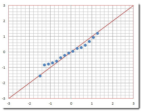
You can use the normal probability plots (i.e. Q-Q plots) as an informal means of assessing the non-normality of a set of data. However, you may need considerable practice before you can judge them with any degree of confidence.
Note: For illustration, we simulated 5 series of random numbers using the Analysis Pack in Excel. Each series has a different underlying distribution: Normal, Uniform, Binomial, Poisson, and Student’s t and F distribution.
Background
Let’s assume we have a data set of a univariate ($\left \{ x_t \right \}$), and we wish to determine whether the data set is well-modeled by a Gaussian distribution.
$$H_o:X\sim N(.)$$ $$H_1:X\neq N(.)$$
Where
- $H_o=$ null hypothesis (X is normally distributed)
- $H_1=$ alternative hypothesis (X distribution deviates from Gaussian)
- $N(.)=$ Gaussian or normal distribution
In essence, the normality test is a regular test of a hypothesis that can have two possible outcomes: (1) rejection of the null hypothesis of normality ($H_o$), or (2) failure to reject the null hypothesis.
In practice, when we can’t reject the null hypothesis of normality, it means that the test fails to find deviance from a normal distribution for this sample. Therefore, it is possible the data is normally distributed.
The problem we typically face is that when the sample size is small, even large departures from normality are not detected; conversely, when your sample size is large, even the smallest deviations from normality will lead to a rejected null.
Normality Tests
How do we test for normality? In principle, we compare the empirical (sample) distribution with a theoretical normal distribution. The measure of deviance can be defined based on distribution moments, a Q-Q plot, or the difference summary between two distribution functions.
Let’s examine the following normality tests:
- Jarque-Bera test
- Shapiro-Wilk test
- Anderson – Darling test
Jarque-Bera
The Jarque-Bera test is a goodness-of-fit measure of departure from normality based on the sample kurtosis and skew. In other words, JB determines whether the data have the skew and kurtosis matching a normal distribution.
The test is named after Carlos M. Jarque and Anil K. Bera. The test statistic for JB is defined as:
$$JB=\frac{n}{6}\left (S^{2}+\frac{K^{2}}{4}\right )\sim{X^{2}_{v=2}}$$
Where
- $S=$the sample skew
- $K=$the sample excess kurtosis
- $n=$the number of non-missing values in the sample
- $JB=$the test statistic; $JB$ has an asymptotic chi-square distribution
Notes: For small samples, the chi-squared approximation is overly sensitive, often rejecting the null hypothesis (i.e. normality) when it is in fact true.

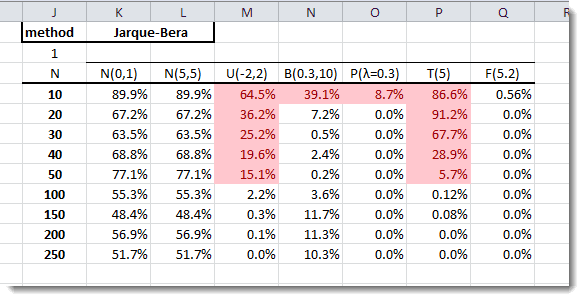
In the table above, we compute the P-value of the normality test (Using the Normality Test function in NumXL). Note that the JB test failed to detect a departure from normality for symmetric distributions (e.g. Uniform and Students) using a small sample size ($n\leq50$).
Shapiro-Wilk
Based on the informal approach to judging normality, one rather obvious way to judge the near linearity of any Q-Q plot (see Figure 1) is to compute its "correlation coefficient."

When this is done for normal probability (Q-Q) plots, a formal test can be obtained that is essentially equivalent to the powerful Shapiro-Wilk test W and its approximation W.
$$W=\frac{\left( \sum_{i=1}^{n} \left( {a_i}{x_{(i)}} \right) \right)^2}{\sum_{i=1}^n(x_{(i)}-\overline{X})^2}$$
Where
- $X_{(i)}=$ the $i^{th}$ order (smallest number in the sample)
- $a_{i}=$ a constant given by $$(a_{1},a_{2},...,a_{n})=\frac{m^{T}V^{-1}}{\sqrt{(m^{T}V^{-1}V^{-1}m)}}$$
- $m=$ the expected values of the order statistics of independent and identical distributed random variables sampled from Gaussian distribution
- $V=$ the covariance matric of ${m}$ order statistics

In the table above, the SW P-values are significantly better for small sample sizes ($n\leq 50$) in detecting departure from normality, but exhibit similar issues with symmetric distribution (e.g. Uniform, Student’s t).
Anderson-Darling
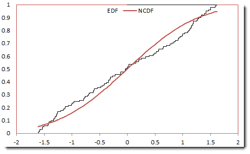
The Anderson-Darling tests for normality are based on the empirical distribution function (EDF). The test statistics is based on the squared difference between normal and empirical:
$$A=-n-\frac{1}{n}\sum_{i=1}^{n}\left [ (2i-1)\ln U_{i}+(2n+1-2i)\ln(1-U_{i}) \right ]$$
In sum, we construct an empirical distribution using the sorted sample data, compute the theoretical (Gaussian) cumulative distribution ($U_{i}$) at each point ($X_{i}$) and, finally, calculate the test statistic

And, in the case where the variance and mean of the normal distribution are both unknown, the test statistic is expressed as follows:
$$A^{*2}=A^{2}\times \left ( 1+\frac{4}{n}-\frac{25}{n^{2}} \right )$$
Note: The AD Test is currently planned for the next NumXL release; we won’t show results here, as you can’t yet reproduce them.
Conclusion
These three tests use very different approaches to test for normality: (1) JB uses the moments-based comparison, (2) SW examines the correlation in the Q-Q plot and (3) AD tests the difference between empirical and theoretical distributions.
In a way, the tests complement each other, but some are more useful in certain situations than others. For example, JB works poorly for small sample sizes (n<50) or very large sample sizes (n>5000).
The SW method works better for small sample sizes (n>3 but less than 5000).
In terms of power, StephensStephens, M. A. (1974). "EDF Statistics for Goodness of Fit and Some Comparisons". Journal of the American Statistical Association 69: 730–737 found AD statistics ($A^{2}$) to be one of the best EDF statistics for detecting departure from normality, even when used with small samples ($n\leq 25$). Nevertheless, the AD test has the same problem with a large sample size, where slight imperfections lead to a rejection of a null hypothesis.
Comments
Article is closed for comments.