Homogeneity

In this issue, the third tutorial in our data preparation series, we will touch on the third most important assumption in time series analysis: Homogeneity, or the assumption that a time series sample is drawn from a stable/homogeneous process.

We’ll start by defining the homogeneous stochastic process and stating the minimum requirements for our time series analysis. Then we demonstrate how to examine the sample data, draw a few observations, and highlight some underlying intuitions behind them.

Background

In statistics, homogeneity is used to describe the statistical properties of a particular data set. In essence, it states that the statistical properties of any part of an overall data set are the same as any other part.

What do we mean by statistical properties? A strict way of looking at homogeneity would involve examining the changes to the whole of the marginal distribution, but time series analysis only demands that we consider the location stability over time (versus trend) and the stability of local fluctuation over time.

What does this mean?

In time series analysis, we are concerned with the stability of the underlying stochastic process over time. Do we have structural changes? If changes exist but go undetected, we find ourselves in one of several difficult situations:

1. The proposed model offers little explanation for the data variation over time
2. The model’s parameter values vary significantly when we re-calibrate using either a subset of the sample or by incorporating new observations
3. In extreme cases, the selection of the best model type or order(s) can be influenced by the selection of sample data

Why do we care?

The objective of time series analysis and modeling is usually the construction of out-of-sample forecasts. How can we generate these forecasts using a model with time-varying parameters? How much confidence can we put in those forecasts? Is the forecast robust? Let’s find out.

Why does it happen?

There are several causes for heterogeneity (opposite of homogeneity) in a time series:

1. The underlying model’s statistical properties are evolving over time. In this case, trying to fit a model with fixed parameter values would not be optimal, despite our best efforts. We need to examine advanced modeling techniques to capture the dynamics of the statistical properties of the process. This, unfortunately, is outside the scope of this paper.
2. The underlying process is not stationary (e.g. possesses trend over time).
3. The underlying process is heteroskedastic where volatility exhibits clustering and mean reversion.
4. The underlying process had undergone few but major structural changes due to exogenous events, such as the passing and enforcement of new relevant laws or a major development in the process itself.

Example 1:

The ozone level in downtown Los Angeles case (refer to the “How does it fit” issue)

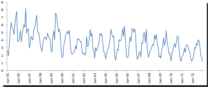
Throughout the sample time between 1955 and 1972, there were two major developments:

1. Rule #76 for gasoline mix and combustion engine design
2. Opening of a freeway to divert traffic from downtown LA

Obviously, those exogenous events affect the number of cars in downtown LA, and consequently the amount of Ozone emitted in the area. One can argue that the process after those events (1972) is not the same as the process in 1960.

Example II:

US Consumer Price Index and its derivative, the inflation rate:

The inflation rate in the US reflects the effectiveness of government public policies, so throughout the sample horizon between 1913 and 2009, it is no surprise that the data characteristics before and after World War II are fundamentally different. Also consider that in the 1970s, the sudden rise in inflation evident in our data reflects a fundamental change (or failure) in public policy.

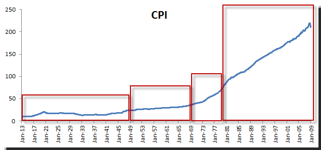
Most importantly, the inflation rate underlying the process after the 1970s is very different than in prior years, for a number of reasons: (1) fundamental changes in public policies and (2) a mandate for the Federal Reserve to fight the inflation rate and unemployment in 1977.

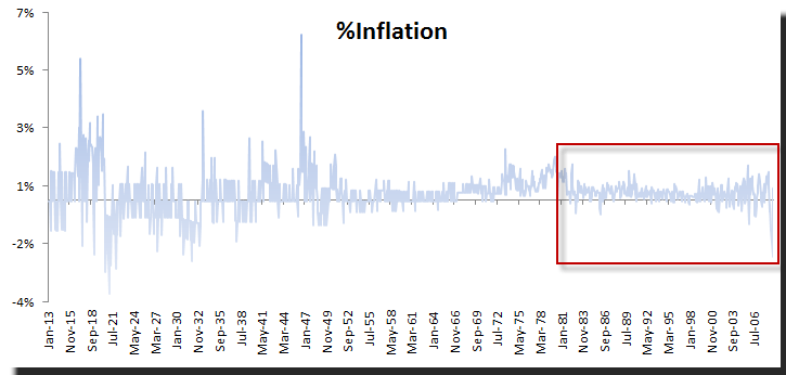
In sum, one may argue that the post-1977 process is very different from the pre-1977 process.

Conclusion

The investigator must bring rich prior knowledge and strong hypotheses about the underlying process structure and its drivers to his interpretation of a data set. The liability of powerful analytical methods is the potential for a rich diversity of alternative solutions that can have very different properties when extrapolated from the situation from which the data was originally sampled.

Checking For Homogeneity

The initial stages in the analysis of a time series may involve plotting values against time to examine the homogeneity of the series in various ways: namely, stability across time (as opposed to a trend) and stability of local fluctuations over time.

In a statistical sense, a test for homogeneity is equivalent to a test of a statistical distribution. In plain English, we wish to detect a change in the underlying distribution. For that, we can examine the distribution moments: mean, variance, skew, and kurtosis for changes.

For time series analysis, we will look into the 1st two moments: mean and variance, and examine any shift over time. Here are few tests to aid us:

• Standard Normal Homogeneity Test (SNHT) :
  Q: Do we have a shift in the mean or variance? $$H_0:r\sim N (0,1)$$ $$H_1: \textrm{There is shift}$$

  Where $r$ are the standardized ratios (an observation’s value compared to the average).

• Pettitt’s Test - detecting a shift in variance - Non-parametric test (i.e. no assumption about the distribution of data).
  Q: Do we have a shift in the variance? When?
  Pettitt's test is an adaptation of the rank-based Mann-Whitney test, which allows you to identify the time at which the shift occurs.
• Tests for detecting a shift in the mean - Non-parametric test (i.e. no assumption about the distribution of data).
  Q: Do we have a shift in the mean? When?
  $$H_0:\mu_t = c$$ $$H_1:\exists\mu_k \neq c$$ Where
  • $H_0$ is the null hypothesis, which states that $x_t$ follows one or more distributions that have the same mean.
  • $H_1$ is the alternative hypothesis, which states that there exists a time k from which the variables change mean.
• Bartles Test (ranked version of Von Neumann ratio test) for randomness –
  Q: Is the sample data random? Do we have patterns?
  • Null Hypothesis $(H_0)$: time series is homogeneous.
  • Alternative hypothesis $(H_1)$: time series is not homogeneous.

Hold on, doesn’t homogeneity sound a lot like stationarity?

Stationarity and homogeneity are closely related; stationarity looks into the stability of the joint distribution $F_x (x_{t_1},x_{t_2},...,x_{t_n})$, while homogeneity examines the stability of the whole marginal distribution over time.

A non-stationary time series is non-homogeneous, but the opposite may not always be true.

My time series is not homogeneous over time; what can I do?

If a homogeneous assumption fails to hold, we need to take a closer look and understand the time series:

1. Is the time series stationary? If so, transform the data to bring it to stationarity.
2. Identify and understand the drivers of the underlying process:
• Do we have exogenous drivers/factors (e.g. laws, events, etc.) that could affect the values of the observations?
• Has the underlying process changed permanently over time?
• Do we expect the exogenous factor to change again in the future?
• When did the process mean or variance change?

In the US CPI example, the change made in 1977 by congress to mandate the Federal Reserve to adopt a public policy to control inflation is a major turning point, and we are inclined to conclude that process underwent a permanent change as a result of that development. In this case, I would disregard all observations before that time.

In the Ozone level in downtown LA example, the opening of a freeway diverting traffic from downtown is a structural change in the underlying process. The same can be said about the laws for gasoline mix and engine design. Again, I would disregard data before the changes took effect, and only concern myself with observations that occur after these events.