Smoothing and filtering are two of the most commonly used time series techniques for removing noise from the underlying data to help reveal the important features and components (e.g., trend, seasonality, etc.). However, we can also use smoothing to fill in missing values and/or conduct a forecast.
In this issue, we will discuss five (5) different smoothing methods: weighted moving average (WMA), simple exponential smoothing, double exponential smoothing, linear exponential smoothing, and triple exponential smoothing.
Why should we care?
Smoothing is often used (and abused) to quickly visualize the data properties (e.g., trend, seasonality, etc.), fit in missing values, and conduct a quick out-of-sample forecast.
Why do we have so many smoothing functions?
As we will see in this paper, each function works for a different assumption about the underlying data. For instance, simple exponential smoothing assumes the data has a stable mean (or at least a slow-moving mean), so simple exponential smoothing will do poorly in forecasting data exhibiting seasonality or a trend.
This paper will go over each smoothing function, highlight its assumptions and parameters, and demonstrate its application through examples.
1. Weighted Moving Average (WMA)
A moving average is commonly used with time-series data to smooth out short-term fluctuations and highlight longer-term trends or cycles. A weighted moving average has multiplying factors to give different weights to data at different positions in the sample window.
$$Y_t=\frac{\sum_{i=1}^N{W_i X_{t-i}}}{\sum_{i=1}^N W_i}$$
Where:
- $W_i$ is the i-th position weight-factor
- $\{X_t\}$ is the original time series
- $\{Y_t\}$ is the smoothed time series
- $Y_t$ uses the prior N-values of $X_t$ observations (i.e. $\{X_{t-1},X_{t-2},\cdots ,X_{t-N}\}$)
The weighted moving average has a fixed window (i.e., N), and the factors are typically chosen to give more weight to recent observations.
The window size (N) determines the number of points averaged at each time, so a larger windows size is less responsive to new changes in the original time series, and small window size can cause the smoothed output to be noisy.
For out of sample forecasting purposes:
$$Y_{T+1}=\sum_{i=1}^N \left ( {w_i X_{T+1-i}}\right )$$ $$Y_{T+2}= w_1 Y_{T+1}+\sum_{i=2}^N \left ( {w_i X_{T+2-i}}\right ) = w_1 \sum_{i=1}^N \left ( {w_i X_{T+1-i}}\right ) + \sum_{i=2}^N \left ( {w_i X_{T+2-i}}\right )$$ $$Y_{T+3}= (w_1^2 +w_2)\sum_{i=1}^N \left ( {w_i X_{T+1-i}}\right ) + w_1 \sum_{i=2}^N \left ( {w_i X_{T+2-i}}\right ) + \sum_{i=3}^N \left ( {w_i X_{T+3-i}}\right )$$ $$Y_{T+4}=(w_1^3+2w_2w_1+w_3)\sum_{i=1}^N \left ( {w_i X_{T+1-i}}\right )+ (w_1^2+w_2)\sum_{i=2}^N \left ( {w_i X_{T+2-i}}\right )+w_1\sum_{i=3}^N \left ( {w_i X_{T+3-i}}\right )+ \sum_{i=4}^N \left ( {w_i X_{T+4-i}}\right )$$
Where:
- $\{w_i\}$ is the normalized weight-factors
Example 1:
Let’s consider monthly sales for Company X, using a 4-month (equal-weighted) moving average.
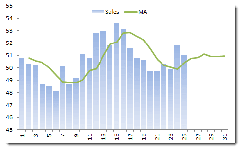
Note that the moving average always lags behind the data, and the out-of-sample forecast converges to a constant value.
Let’s try to use a weighting scheme (see below) that emphasizes the latest observation.
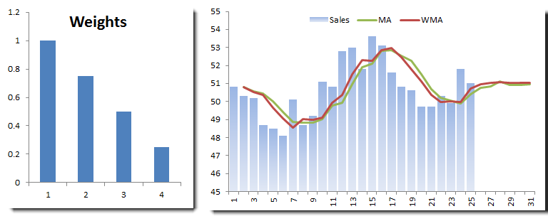
We plotted the equal-weighted moving average and WMA on the same graph. The WMA seems more responsive to recent changes, and the out-of-sample forecast converges to the same value as the moving average.
Example 2:
Let’s examine the WMA in the presence of trend and seasonality. For this example, we’ll use the international passenger airline data. The moving average window is 12 months.
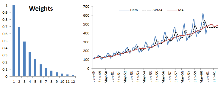
The MA and the WMA keep pace with the trend, but the out-of-sample forecast flattens. Furthermore, although the WMA exhibits some seasonality, it is always lagging behind the original data.
2. Simple (Brown's) Exponential Smoothing
Simple exponential smoothing is similar to the WMA except that the window size is infinite, and the weighting factors decrease exponentially.
$$Y_1=X_1$$ $$Y_2=(1-\alpha)Y_1+\alpha X_1=X_1$$ $$Y_3=(1-\alpha)Y_2+\alpha X_2=(1-\alpha)X_1+\alpha X_2$$ $$Y_4=(1-\alpha)Y_3+\alpha X_3=(1-\alpha)^2 X_1+\alpha (1-\alpha) X_2+\alpha X_3$$ $$Y_5=(1-\alpha)^3 X_1+\alpha (1-\alpha)^2 X_2+\alpha (1-\alpha) X_3 + \alpha X_4$$ $$Y_{T+1}=(1-\alpha)^T X_1+\alpha \sum_{i=1}^T (1-\alpha)^{T-i}X_{i+1}$$ $$\cdots$$ $$Y_{T+m}=Y_{T+1}$$
Where:
- $\alpha$ is the smoothing factor ($0 \prec \alpha \prec 1$
As we have seen in the WMA, the simple exponential is suited for time series with a stable mean or a very slow-moving mean.
Example 1:
Let’s use the monthly sales data (as we did in the WMA example).
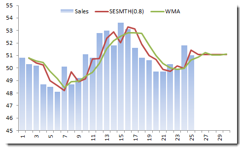
In the example above, we chose the smoothing factor to be 0.8, which begs the question: What is the best value for the smoothing factor?
Estimating the best $\alpha$ value from the data
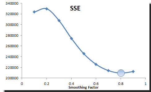
In practice, the smoothing parameter is often chosen by a grid search of the parameter space; that is, different solutions for $\alpha$ are tried, starting with, for example, $\alpha=0.1$ to $\alpha = 0.9$, with increments of 0.1. Then $\alpha$ is chosen to produce the smallest sums of squares (or mean squares) for the residuals (i.e., observed values minus one-step-ahead forecasts; this means squared the error is also referred to as ex-post mean squared error (ex-post MSE for short).
Using the TSSUB function (to compute the error), SUMSQ, and Excel data tables, we computed the sum of the squared errors (SSE) and plotted the results:
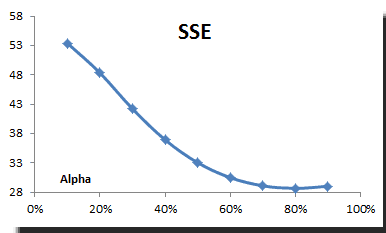
The SSE reaches its minimum value around 0.8, so we picked this value for our smoothing.
3. Double (Holt's) Exponential Smoothing
Simple exponential smoothing does not do well in the presence of a trend, so several methods devised under the “double exponential” umbrella are proposed to handle this type of data.
NumXL supports Holt’s double exponential smoothing, which take the following formulation:
$$S_1=X_1$$ $$B_1=\frac{X_T-X_1}{T-1}$$ $$S_{t>1}=\alpha X_t + (1-\alpha)(S_{t-1}+B_{t-1})$$ $$B_{t>1}=\beta (S_t - S_{t-1})+(1-\beta)B_{t-1}$$ $$Y_t=\left\{\begin{matrix} S_t+B_t & t<T\\ S_T+m\times B_T & t=T+m \end{matrix}\right.$$
Where
- $\alpha$ is the smoothing factor ($0 \prec \alpha \prec 1$)
- $\beta$ is the trend smoothing factor ($0 \prec \beta \prec 1$)
Example 1:
Let’s examine the international passengers’ airline data
We chose an Alpha value of 0.9 and a Beta of 0.1. Please note that although double smoothing traces the original data well, the out-of-sample forecast is inferior to the simple moving average.
How do we find the best smoothing factors?
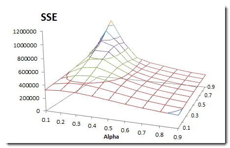
We take a similar approach to our simple exponential smoothing example but modified for two variables. We compute the sum of the squared errors; construct a two-variable data table, and pick the alpha and beta values that minimize the overall SSE.
4. Linear (Brown's) Exponential Smoothing
This is another method of double exponential smoothing function, but it has one smoothing factor:
$$S_1^{'}=X_1$$ $$S_1^{''}=X_1$$ $$S_{t>1}^{'}=\alpha X_t + (1-\alpha)S_{t-1}^{'}$$ $$S_{t>1}^{''}=\alpha S_{t}^{'}+(1-\alpha)S_{t-1}^{''}$$ $$a_{1<t<T}=2 S_{t}^{'}-S_t^{''}$$ $$b_{1<t<T}=\frac{\alpha}{1-\alpha}\times (S_t^{'}-S_t^{''})$$ $$Y_{T+m}=a_T+m\times b_T$$
Where
- $\alpha$ is the smoothing factor ($0 \prec \alpha \prec 1$)
Brown’s double exponential smoothing takes one parameter less than Holt-Winter’s function, but it may not offer as good a fit as that function.
Example 1:
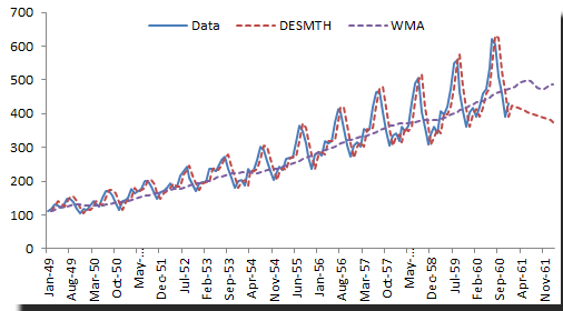
Let’s use the same example in Holt-Winter’s double exponential and compare the optimal sum of the squared error.
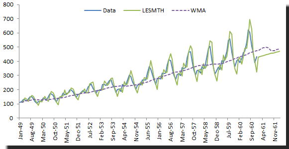
Brown’s double exponential does not fit the sample data as well as the Holt-Winter’s method, but the out-of-sample (in this particular case) is better.
How do we find the best smoothing factor ($\alpha$)?
We use the same method to select the alpha value that minimizes the sum of the squared error. For the example sample data, the alpha is found to be 0.8.
5. Triple (Holt-Winter’s) Exponential Smoothing
The triple exponential smoothing takes into account seasonal changes as well as trends. This method requires 4 parameters:
- $\alpha$: the smoothing factor
- $\beta$: the tend smoothing factor
- $\gamma$: the seasonality smoothing factor
- $\mathrm{L}$: the season Length
The formulation for triple exponential smoothing is more involved than any of the earlier ones. Please, check our online reference manual for the exact formulation.
Example:
Using the international passengers’ airline data, we can apply winter’s triple exponential smoothing, find optimal parameters, and conduct an out-of-sample forecast.
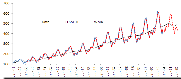
Obviously, Winter’s triple exponential smoothing is best applied for this data sample, as it tracks the values well, and the out-of-sample forecast exhibits seasonality (L=12).
How do we find the best smoothing factor ($\alpha,\beta,\gamma$)?
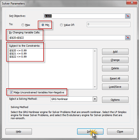
Again, we need to pick the values that minimize the overall sum of the squared errors (SSE), but the data tables can be used for more than two variables, so we resort to the Excel solver:
(1) Setup the minimization problem, with the SSE as the utility function
(2) The constraints for this problem
$$ 0 < \alpha < 1 $$ $$ 0 < \beta < 1 $$ $$ 0 < \gamma < 1 $$
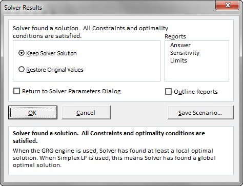
(3) Launch the Solver and initialize utility and constraints.
(4) The solver searches for the optimal solution, ultimately prompting its completion.
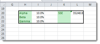
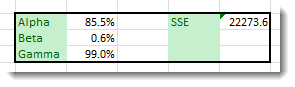
(5) The optimal values are:
Conclusion
In this paper, we demonstrated the use of different smoothing functions, finding optimal parameters and projecting forecasts for each while demonstrating scenarios in which particular smoothing methods may not be appropriate.
You should always visually examine the data for signs of seasonality or linear trend and select a smoothing method based on your findings.
In practice, smoothing-based forecasts are often used for one-to-few steps, and they are relatively accurate (given their simplicity) compared to more sophisticated models.
Support Files
Comments
Article is closed for comments.