NumXL Cookbook - GLM with Binary Data

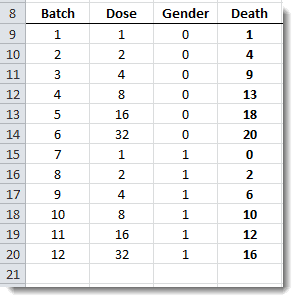
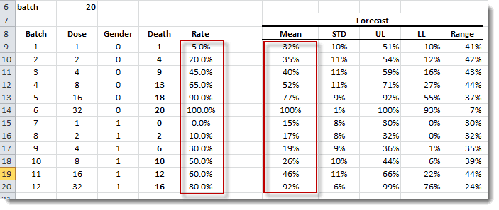
In this tutorial, we will use sample data gathered during a clinical trial of a new chemical/pesticide on tobacco Budworms. The subjects (i.e. Budworms) are grouped into batches of 20 and exposed to different doses of the chemical. The results are summarized below:

Data preparation

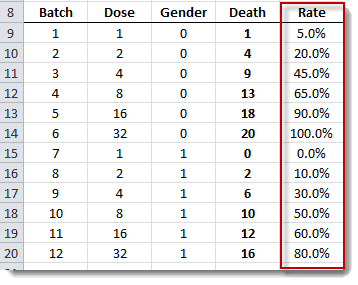
Our objective here is to model (and forecast) the effectiveness of the new chemical using different dosages and explain, to some extent, any variation based on the gender of the budworm. Furthermore, we want to express the results in terms of the worm mortality rates (i.e. probability).

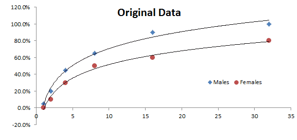
We plot the data into two separate curves: males and females. It is apparent that the mortality rate is affected by two factors: gender and dosage.

We will make two assumptions: (1) the results for each trial (i.e. batch) are drawn from a Binomially distributed population; we would like to estimate p - the probability of success (i.e. worm’s death). The probability (p) is allowed to vary across different trials (batches). (2) The probability of success is affected by two factors: the gender of the subject and the administered dosage of the drug.

Based on these two assumptions, we would model this relationship:

$$P=f(X,Y)=E[p|X,Y]$$

Modeling

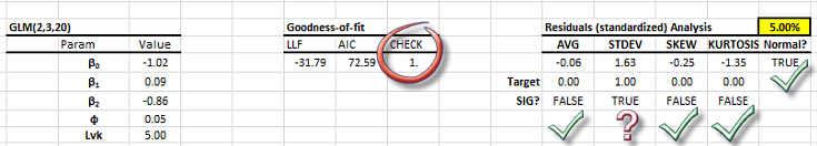
We are ready now to propose a statistical model: the generalized linear model in Excel with residuals following the Binomial distribution.

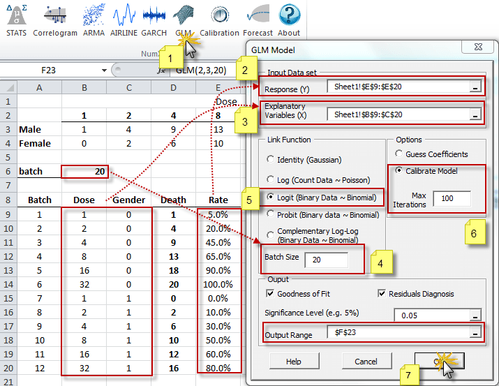
For now, we choose “Logit” as our link (transform) function, specify the trial or batch size(20), and instruct the Wizard to calibrate (i.e. compute optimal values for the coefficients). Leave the Goodness-of-fit and residual diagnosis options checked.

Calibration

In this case, the Generalized Linear Model in Excel (GLM) Wizard has calibrated the model’s coefficients, so we can skip this step.

But, in the event we wish to experiment with different link functions: LOGIT, PROBIT or LOG-LOG, then we need to re-calibrate the model. To do so, we can either:

1. Create a new model with the wizard, or,
2. Change the “Lvk” parameter in an existing model table, and run the calibration using the NumXL toolbar

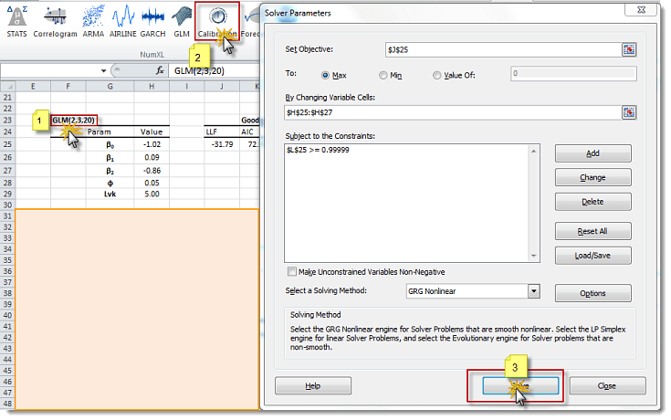
Step 1: Select the cell that acts as a header for the model table

Step 2: Click on the calibration icon/menu (Excel 2003)

Step 3: Click on the “Solve” button in the Solver window

Forecast

Once the model is calibrated, and we are happy with the residuals, we can use it to construct our forecast mean (and the confidence interval around it).

Using the NumXL function (GLM_FORE), we can compute the mean. Using GLM_FORECI, we can compute the upper and lower limit of the confidence interval.

Plotting the data again (actual) versus the model values.

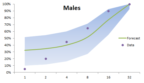
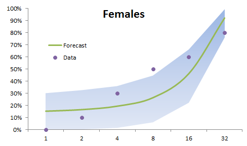
The dots represent the sample data, while the centerline is the forecast mean. The shaded regions in the graphs are the 95% confidence intervals.

Tutorial Video