Discrete Fourier Transform (DFT)

This is the first tutorial on time series spectral analysis. In this entry, we examine the Discrete Fourier Transform (DFT) and its inverse, as well as data filtering using DFT outputs. The DFT is basically a mathematical transformation and maybe a bit dry, but we hope that this tutorial will leave you with a deeper understanding and intuition through the use of NumXL functions and wizards.

In future entries, we will dedicate more time to discrete data filters, their construction, and of course, application.

Background

You have probably occasionally transformed your data to stabilize the variance (e.g. log transform) or to improve the distribution of the values in the sample data.

$$x_t=\{ x_1,x_2, \cdots , x_T \}$$

$$y_t=\log(x_t)$$

$$y_t=\{y_1,y_2, \cdots , y_T\}$$

In mathematics, the discrete Fourier transform (DFT) converts a finite list of equally-spaced samples of a function into a list of coefficients of a finite combination of complex sinusoids, ordered by their frequencies, which have those same sample values. DFT converts the sampled function from its original domain (often time or position along a line) to the frequency domain.

In sum, the Fourier transform has the following properties:

1. The transformed data is no longer in the time domain.
2. The transformation operates on the whole data set. It is not a point-by-point transformation as we have seen with earlier transformations in the time domain.
   
   $$x_t=\{ x_1,x_2, \cdots , x_T \}$$
   $$Y= \mathcal{F}(\{ x_1,x_2, \cdots , x_T \})$$
   $$Y=\{ y_1,y_2, \cdots , x_k \}$$
   $$\{ x_1,x_2, \cdots , x_T \} = \mathcal{F}^{-1}(\{ y_1,y_2, \cdots , x_k \})$$
3. The transformed data is complex (not real-valued).

What is the Discrete Fourier Transform (DFT)?

In plain words, the discrete Fourier transform decomposes the input time series into a set of cosine functions.

$$x_m=\frac{1}{N}\sum_{k=1}^N A_k \times \cos(\phi_k+k\times \omega \times m)$$

So, you can think of the k-th output of the DFT as the $A_k \angle \phi_k$. The $A_k$ is referred to as the amplitude and the $\phi_k$ as the phase (in radians).

The input time series can now be expressed either as a time-sequence of values or as a frequency-sequence of $[A_k \angle \phi_k]$. pairs. Knowing the set of $[A_k \angle \phi_k]$, we can recover the exact input time series.

What is $\omega$?

$\omega$ is the fundamental or the principal radian frequency. IT is expressed as follows:

$$\omega = \frac{2\pi}{T}$$

Where:

• $T$ is the number of observations in the equally-spaced input time series.

What is N?

N is the number of $[A_k \angle \phi_k]$ pairs we need to have, so we can recover the original input time series with a floor value of $\frac{T}{2}$.

Note that the zero-frequency component (i.e. k=0) is always real-value, and in the case of even-sized time series, the last frequency component is also real-value, which brings the total number of values (amplitude and phase) to T. There is no gain or loss of information or storage requirement because of this transform.

Finally, note that
$$A_k \angle \phi_{T-k} = A_k \angle -\phi_k$$

$$A_k \angle \phi_{T+k} = A_k \angle \phi_k$$

In essence, only the values of the first $\left \lfloor \frac{T}{2} \right \rfloor$ frequency components are needed, whereas the rest can be easily implied from them. Furthermore, the DFT values are periodic with a cycle length of $T$.

Why decompose time series data into a series of cosine functions?

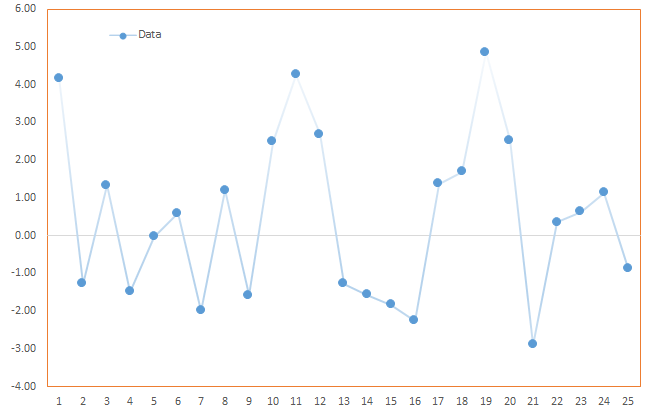
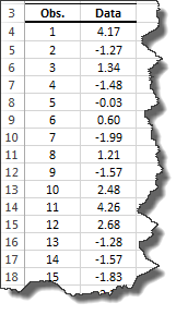
Consider the following time series $\{x_1, x_2, \cdots , x_{25} \}$:

Now, let’s compute the time series using a subset of the frequency sequence:

Case 1: Using the zero frequency component

Using the zero frequency component:

$$x_m^{(0)}= \frac{A_o}{T}=\frac{A_o}{25}$$

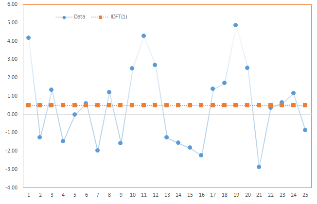
Using the zero frequency, we get the long-run average of the time series.

Case 2: Using first frequency component (k=1)

$$ x_m^{(0)}= \frac{A_o}{T}$$

$$\omega = \frac{2\pi}{T}$$

$$x_m^{(1)}= \frac{1}{T} (A_o + A_1 \cos (\phi_1+\omega \times m)= x_m^{(0)} + \frac{A_1}{T}\cos (\phi_1+\omega \times m)$$

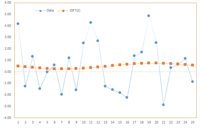
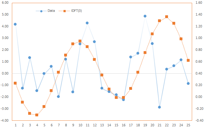
Note that the graph on the right is essentially the same as the one on the left, but with plotted using the right-hand-side axis scale.

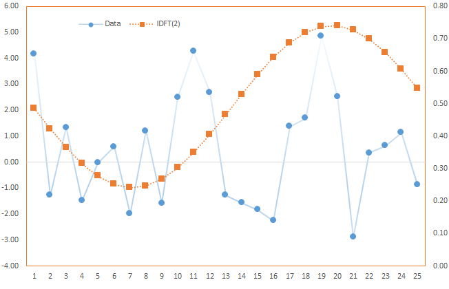
Case 3: Using first and second frequency components (k=2)

$$x_m^{(0)}= \frac{A_o}{T}=\frac{A_o}{25}$$

$$\omega = \frac{2\pi}{T}$$

$$ x_m^{(1)}= \frac{1}{T} (A_o + A_1 \cos (\phi_1+\omega \times m)= x_m^{(0)} + \frac{A_1}{T}\cos (\phi_1+\omega \times m)$$

$$x_m^{(2)}= \frac{1}{T} (A_o + A_1 \cos (\phi_1+\omega \times m ) + A_2 \cos (\phi_2+ 2\omega \times m )) $$

$$x_m^{(2)} = x_m^{(1)} + \frac{A_2}{T}\cos (\phi_2 + 2 \omega \times m)$$

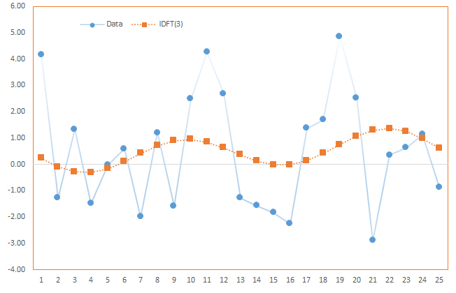
Note, $x_m^{(2)}$ is closer to the original time series than $x_m^{(1)}$ due to the added cosine function, but $x_m^{(1)}$ is smoother.

In essence, the process of recovering the original time series from the subset is similar to time series smoothing, but without the drawback of the lag effect.

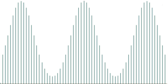
Case 4: Using the first 8 frequency components (k=8)

$$x_m^{(0)}= \frac{A_o}{T}$$

$$x_m^{(1)}= x_m^{(0)} + \frac{A_1}{T}\cos (\phi_1+\omega \times m)$$

$$x_m^{(2)}= x_m^{(1)} + \frac{A_2}{T}\cos (\phi_2+ 2 \omega \times m)$$

$$x_m^{(3)}= x_m^{(2)} + \frac{A_3}{T}\cos (\phi_3+ 3 \omega \times m)$$

$$\cdots$$

$$x_m^{(8)}= x_m^{(7)} + \frac{A_8}{T}\cos (\phi_8+ 8 \omega \times m)$$

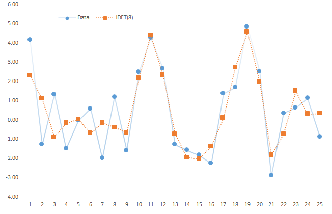
In sum, by decomposing the input time series into cosine functions, we can separate the component(s) attributed to noise (high frequency), uncover periodicity, and find a long-run value for the process.

Process

First, let’s organize our input data. We can start by placing the values of the sample data in a separate column.

Now we are ready to construct our DFT output table. First, select the empty cell in your worksheet where you wish the output table to be generated, then locate and click on the “Fourier” icon in the NumXL tab (or toolbar).

The DFT Wizard pops up.

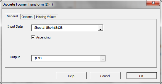
Select the cell range for the values of the input variable.

Finally, once we select the input data (X) cells range, the “Options” and “Missing Values” tabs become available (enabled).

Next, select the “Options” tab:

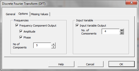
Initially, the tab is set to the following values:

• “Frequency Component Output” is checked. Leave this option checked.
  • The Amplitude and Phase options are checked. Leave those options checked as well.
  • The number of components corresponds to the size of the output table. Set this value to five (5) to generate the first five frequency components.
• On the right side, “Input Variable Output” is unchecked. Check this option to generate back the input time series using a subset of the frequency components.
  • Under “No. of Components”, set this value to 4. You can change this value later on in the output table.

Now, click on the “Missing Values” tab.

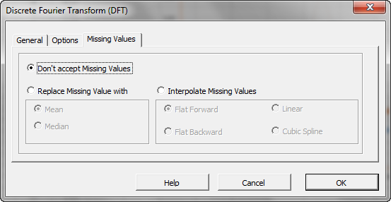
In this tab, you can select an approach to handle missing values in the data set (X’s). By default, the DFT wizard does not allow any missing value in the analysis.

This treatment is a good approach for our analysis, so let’s leave it unchanged.

Output

Now, click “OK” to generate the output tables.

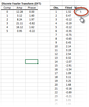
The first table (on the left), displays the amplitude and phase (in radians) for different frequency components (i.e. cosine functions). Note that component zero has zero phase.

In the second table, it carries on the inverse Fourier transform using a subset of the frequencies.

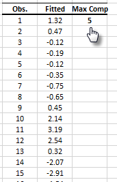
If you wish to change the number of components, simply edit the number in the cell table, and the values under the “Fitted” title will be recalculated.

Conclusion

In this tutorial, we presented the interpretation of the discrete Fourier transform (DFT) and its inverse (IDFT), as well as the process to carry out the related calculation in Excel using NumXL’s add-in functions.

Where do we go from here?

Using DFT, we constructed an analytical formula representation for the input time series.

One direct application that we can think of is to compute values for the new intermediate observation or to alter the sampling frequency (i.e. up-sample) and introduce a new time series.

But what about missing values? What if we don’t have a fixed sampling rate? Different types of Fourier transforms are available (e.g. non-uniform time discrete Fourier transform (NUT-DFT)) to handle unequally spaced input time series, which generate a finite discrete set of frequencies. This will prove to be useful for imputing intermediate missing values using the dynamics of the whole data set, rather than adjacent observations, as is the case in interpolation or Gaussian bridge methods.

The time series spectrum contains a significant amount of information, which we barely scratched in this tutorial. In our next entry, we will look at the discrete filter (operator) definition in both the time and frequency domain and its application to our time series analysis/modeling.