Regression Analysis 101

This is the first entry in what will become an ongoing series on regression analysis and modeling. In this tutorial, we will start with the general definition or topology of a regression model, and then use the NumXL program to construct a preliminary model. Next, we will closely examine the different output elements in an attempt to develop a solid understanding of regression, which will pave the way to more advanced treatment in future issues.

In this tutorial, we will use a sample data set gathered from 20 different salespersons. The regression model attempts to explain and predict a sales person’s weekly sales (dependent variable) using two explanatory variables: Intelligence (IQ) and extroversion.

Data Preparation

First, let’s organize our input data. Although not necessary, it is customary to place all independent variables (X’s) on the left, where each column represents a single variable. In the right-most column, we place the response or the dependent variable values.

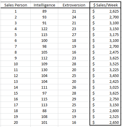
In this example, we have 20 observations and two independent (explanatory) variables. The amount of weekly sales is the response or dependent variable.

Process

Now we are ready to conduct our regression analysis. First, select an empty cell in your worksheet where you wish the output to be generated, then locate and click on the regression icon in the NumXL tab (or toolbar).

Now the Regression Wizard will appear.

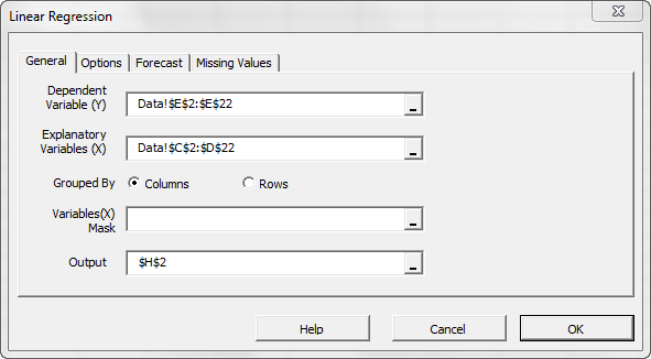
Select the cell range for the response/dependent variable values (i.e. weekly sales). Select the cell range for the explanatory (independent) variables values.

Finally, once we select the X and Y cells range, the “options,” “Forecast” and “Missing Values” tabs will become available (enabled).

Next, select the “Options” tab.

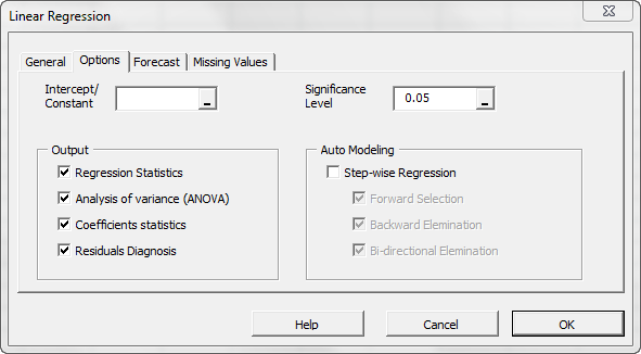
Initially, the tab is set to the following values:

• The regression intercept/constant is left blank. This indicates that the regression intercept will be estimated by the regression. To set the regression to a fixed value (e.g. zero (0)), enter it there.
• The significance level (aka. ) is set to 5%.
• In the output section, the most common regression analysis is selected.
• For auto-modeling, let’s leave it unchecked. We will discuss this functionality in a later issue.

Now, click on the “Missing Values” tab.

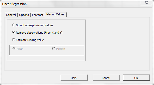
In this tab, you can select the approach to handle missing values in the data set (X and Y). By default, any missing value found in X or in Y in any observation would exclude the observation from the analysis.

This treatment is a good approach for our analysis, so let’s leave it unchanged.

Now, click “Ok” to generate the output tables.

Analysis

Let’s now examine the different output tables more closely.

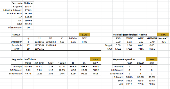
1. Regression Statistics

In this table, a number of summary statistics for the goodness-of-fit of the regression model, given the sample, is displayed.

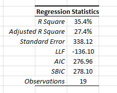
1. The coefficient of determination (R square) describes the ratio of variation in Y described by the regression.
2. The adjusted R-square is an alteration of R square to take into account the number of explanatory variables.
3. The standard error ($\sigma$) is the regression error. In other words, the error in the forecast has a standard deviation of around \$332.
4. Log-likelihood function (LLF), Akaike information criterion (AIC), and Schwartz/Bayesian information criterion (SBIC) are different probabilistic measures for the goodness of fit.
5. Finally, “Observations” is the number of non-missing observations used in the analysis.

2. ANOVA

Before we can seriously consider the regression model, we must answer the following question:

The regression model we have hypothesized is:

$$Y_i=\hat Y_i+e_i =\alpha + \beta_1\times X_{1,i}+\beta_2\times X_{2,i}+e_i$$ $$e_i\sim \textrm{i.i.d}\sim N(0,\sigma^2)$$

Where

• $\hat Y_i$ is the estimated value for the i-th observation.
• $e_i$ is the error term for the i-th observation.
• $e_i$ iis assumed to be independent and identically distributed (Gaussian).
• $\sigma^2$ is the regression variance (standard error squared).
• $\beta_1 ,\beta_2$ are the regression coefficients.
• $\alpha$ is the intercept or the constant of the regression.

Alternatively, the question can be stated as follows:

$$H_o:\beta_1=\beta_2=0$$ $$H_1:\exists\beta_k\neq 0$$ $$1\leqslant k\leqslant 2$$

The analysis of variance (ANOVA) table answers this question.

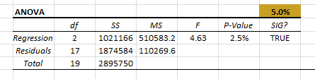
In the first row of the table (i.e. “Regression”), we compute the test-score (F-Stat)and P-Value, then compare them against the significance level ($\alpha$). In our case, the regression model is statistically valid, and it does explain some of the variations in values of the dependent variable (weekly sales).

The remaining calculations in the table are simply to help us to get to this point. To be complete, we described its computation, but you can skip that to the next table.

• $\textrm{df}$ is the degrees of freedom. (For regression, it is the number of explanatory variables ($p$ ). For the total, it is the number of non-missing observations minus one $\left(N-1\right)$ , and for residuals, it is the difference between the two ($N-p-1$ )).
• Sum of squares (SS)
  $$SSR=\sum_{i=1}^N(\hat Y_i - \bar Y)^2$$ $$SST=\sum_{i=1}^N(Y_i - \bar Y)^2$$ $$SSE=\sum_{i=1}^N(Y_i - \hat Y_i)^2$$
• Mean Square (MS):
  $$MSR=\frac{SSR}{p}$$ $$MSE=\frac{SSE}{N-p-1}$$
• Test statistics:
  $$F=\frac{MSR}{MSE}\sim F_{p,N-p-1}(.)$$

3. Residuals Diagnosis Table

Once we confirm that the regression model explains some of the variations in the values of the response variable (weekly sales), we can examine the residuals to make sure that the underlying model’s assumptions are met.

$$Y_i=\hat Y_i+e_i =\alpha + \beta_1\times X_{1,i}+\beta_2\times X_{2,i}+e_i$$ $$e_i\sim \textrm{i.i.d}\sim N(0,\sigma^2)$$

Using the standardized residuals (\tex>\frac{e_i}{\sigma_i}$), we perform a series of statistical tests to the mean, variance, skew, excess kurtosis, and finally, the normality assumption.

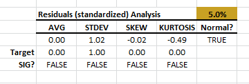
In this example, the standardized residuals pass the tests with 95% confidence.

4. Regression Coefficients table

Once we establish that the regression model is significant, we can look closer at the regression coefficients.

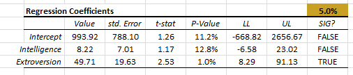
Each coefficient (including the intercept) is shown on a separate row, and we compute the following statistics:

• Value (i.e. $\alpha,\beta_1,\cdots$)
• Standard error in the coefficient value.
• Test score (T-stat) for the following hypothesis:
  $$H_o:\beta_k=0$$ $$H_1:\beta_k \neq 0$$
• The P-Values of the test statistics (using Student’s t-distribution).
• Upper and lower limits of the confidence interval for the coefficient value.
• A reject/accept the decision for the significance of the coefficient value.

In our example, only the “extroversion” variable is found significant while the intercept and the “Intelligence” are not found significant.

Conclusion

In this example, we found that the regression model is statistically significant in explaining the variation in the values of the weekly sales variable, it satisfies the model’s assumptions, but the value of one or more regression coefficients is not significantly different from zero.

What do we do now?

There may be a number of reasons why this is the case, including possible multicollinearity between the variables or simply that one variable should not be included in the model. As the number of explanatory variables increases, answering such questions gets more involved, and we need further analysis.

We will cover this particular issue in a separate entry of our series.

Tutorial Video