Module 3 - Smoothing

In module one (1), we demonstrated the data preparation phase of time series analysis. In module two (2), we described a few steps to calculate numerous summary statistics and verify the significance of their values.

In this module, we will walk you through time series smoothing in Excel using NumXL functions and tools. For sample data, we’ll use the S&P 500 weekly closing prices between January 2009 and July 2012.

NumXL supports numerous smoothing functions, but each function assumes a particular characteristic of the sample data.

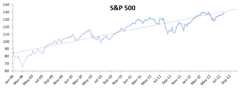
Let’s consider the S&P 500 weekly close price time series between Jan 2009 and July 2012. The time series exhibits a trend over time.

Using equally-weighted moving average (WMA) with a window size of 4 weeks, forecasting into the next 12 weeks, we find:

The WMA keeps pace with the original data, but it is lagging. Furthermore, the out-of-sample forecast is flat.

Assuming the trend is deterministic (non-stochastic), we can use Holt-Winter’s double exponential smoothing functions (DESMTH).

The double exponential smoothing function used optimal values for the smoothing parameters of the exponential smoothing function tracks the data pretty well and the forecast looks in line with the original curve. Is this it? Did we find a crystal ball that tells us where the price will be each week? Not quite!

Earlier, we made the assumption that the trend is deterministic (non-stochastic), but the price is more like a random-walk process, so the trend we observe is just an anomaly that can occur in the random-walk.

Proof!

The Augmented Dickey-Fuller unit-root test (ADF Test) in NumXL can test for the presence of a unit-root (i.e., random-walk) in the presence of drift and/or trend.

$$(1-L)y_t=\triangledown y_t =\alpha + \gamma y_{t-1}+\beta \times t + \cdots$$

The ADF test is basically $H_o:\gamma = 0$.

The unit-root existence is confirmed in all 3 different formulations:

• no constant ($\triangledown y_t =\gamma y_{t-1}+ \epsilon_t$).
• constant ($\triangledown y_t =\alpha + \gamma y_{t-1}+ \epsilon_t$).
• constant+trend ($\triangledown y_t =\alpha + \gamma y_{t-1}+\beta \times t+ \epsilon_t$).

The time series is integrated (i.e., has a unit-root), so we need to take the first difference to stabilize (i.e., make stationary) the input data:

$$z_t = (1-L)y_t=\triangledown y_t$$

Support Files