General Exponential Smoothing (GESMTH) with trend in Excel

Scene 1:

Hello and welcome to the exponential smoothing tutorial series. In this tutorial, we’ll introduce the latest addition to the exponential smoothing functions family – The General Exponential Smoothing Function (GESMTH).

The General Exponential Smoothing Function not only supports prior smoothing models covered by the Simple, double, and triple exponential smoothing functions, but it implements additional types for trend and seasonal components. Furthermore, the General Exponential Smoothing Function supports data prior-transformation and Chatfield correction/adjustment for 1 st order autocorrelation in the forecast errors. In short, the general exponential smoothing function is the ultimate tool in our arsenal to smooth your data, and project forecast.

In this video, we will cover the smoothing models of non-seasonal trending data set using the different trend types and built-in automatic optimization for the smoothing parameters. We will use the annual net power generation in the US using natural gas as fuel between 1949-2016. The data was sourced from US Energy Information Agency, and units are expressed in millions of MegaWatt Hours.

Scene 2:

Examine the plot of data over time, and notice the annual net power generation using natural gas:
- It does not exhibits seasonality
- It grows rapidly in a nonlinear fashion in the years post-1988.

However, the growth is not perfect. Is this pattern? Maybe! Now, we have an idea of what we dealing with, so let’s begin! For illustration, we list the input arguments of the general exponential smoothing function in cells D1- D11. Select cell D18

Scene 3:

Type in the function name – GESMTH in the cell or in the equation toolbar. Note that the auto-complete feature in Microsoft Excel will help find the correct function.

Scene 4:

Once you find the General Exponential Smoothing function, click on the “fx” button located on the left of the equation toolbar. This will invoke the “function arguments dialog” for the General Exponential Smoothing Function.

Scene 5:

First, let’s specify the input cells range.

Scene 6:

Then lock the starting cell reference by pressing F4.

Scene 7:

In the order field, specify 1 (or True) for the time order in the series. This designates that the 1st observation in the input series corresponds to the earliest date.

Scene 8:

For the level-smoothing parameter alpha, you can type in a value between 0 and 1, leave blank, or reference an existing cell.

In this example, let’s reference the value in D1.

Scene 9:

And, lock the cell reference by pressing F4

Scene 10:

For the trend-smoothing parameter (beta), you can also type in a value between 0 and 1, leave blank, or reference an existing cell.

In this example, let’s reference the value in D2.

Scene 11:

Lock the cell reference by pressing F4.

Scene 12:

For Gamma or seasonality indices smoothing parameters, you may type a value between 0 and 1, leave blank, or reference the existing cell in your worksheet.

For consistency, let’s reference the value in D3.

Scene 13:

Lock the cell reference by pressing F4.

Scene 14:

Now, for the trend damping coefficient (Phi), you may type a value between 0 and 1, leave blank, or reference a cell in your worksheet.

Let’s reference the value in D4.

Scene 15:

Lock the cell reference by pressing F4.

Scene 16:

For the parameter value of Chatfield’s autocorrelation correction term (aka Lambda), you may type a value between -1 and 1, leave blank, or reference a cell in your worksheet.

Let’s reference the value in D5.

Scene 17:

Lock the cell reference by pressing F4.

Scene 18:

For trend-type, you need to choose a value from 0 (no trend) to 4 (damped-multiplicative), leave blank (aka no trend), or reference a cell in your worksheet.

Again, let’s reference another cell: D6.

Scene 19:

Lock the cell reference by pressing F4.

Scene 20:

For seasonality type argument, you may leave blank indicating nonseasonal, enter 0, or reference a cell in the spreadsheet.

For consistency with the rest of the arguments, let’s reference D7.

Scene 21:

Lock the cell reference by pressing F4

Scene 22:

For seasonal length, you may leave blank (no seasonality), type in a value (e.g. 1), or reference a cell.

Let’s reference the value in cell D8.

Scene 23:

Lock the cell reference by pressing F4

Scene 24:

For enabling/disabling the built-in optimizer, you may type in True/False, leave blank (disabled), or reference the value in D9

Scene 25:

Lock the cell reference by pressing F4

Scene 26:

For enabling/disabling Chatfield’s autocorrelation correction, enter a True/False, leave blank, or reference the value in D10

Scene 27:

Lock the cell reference by pressing F4

Scene 28:

For prior-data log transform, reference the value in cell D11

Scene 29:

Lock the cell reference by pressing F4

Scene 30:

For the forecast time, we will be forecasting the value at the end of the input data. So, set T to zero, or better yet, reference a cell in column A, so we can change it after the end of the input data.

Scene 31:

Lock the cell for column movement, by hitting F4 until the dollar sign is showing at the left.

Scene 32:

For return type, leave blank or type in zero (0) for "forecast".

Then, click OK.

Scene 33:

The function returns #N/A since we don’t have enough data.

Scene 34:

Copy the formulas to the cells below it, even after the end of the sample data. Don’t worry about the empty cells picked up after the end of the input data, the function will ignore them.

Scene 35:

Let’s plot the optimized one-step smoothing forecast. The general exponential smoothing forecast follows the data pretty well.

Scene 36:

Before we can compare other smoothing models, let’s quantify the forecasting accuracy of the new series. For this illustration, we will use three forecast performance measures: for an absolute measure, we will use mean-squared-error (MSE), for percentage error, we choose symmetric mean absolute percentage error (MAPE), and for a relative scaled error (relative to naïve model), we will use the mean absolute scaled error (MASE). Those functions are part of NumXL and are available as a worksheet function.

Scene 37:

First, let’s examine a no-trend model (aka Brown’s simple exponential smoothing). Set the trend type to 0 (i.e. no trend). The worksheet auto-calculates all values, and the plot reflects the new series. It does not look very good.

Looking further to the forecast accuracy measure:
- MASE states it performs worse than plain naïve forecast.
- MAPE shows that the average percentage error is around 8%.

Scene 38:

OK, let’s add a deterministic additive (linear) trend (aka Holt’s double exponential smoothing). Set the trend type to 1 (i.e. additive trend) in D6. Again, the worksheet recalculates all forecast values, and the graph is updated It looks better than earlier.

Examining the accuracy measure:
- MASE shows it performs better than the naïve model (6% better)
- MAPE shows the same average absolute error.

Scene 39:

Intuitively, we don’t really believe the trend is going to last forever. At some point, the trend will start to level down. Let’s try a damped-additive type of trend. Set the trend type value to 2 in cell D6. Once Excel finishes recalculating the new forecast values, the graph is updated. The new forecast values look better, and both the MASE (92%) and MAPE (7%) improve. Interesting! It seems applying some common-sense intuition is paying off.

Scene 40:

Looking again at the raw data, the growth in net power generation post-1989 follows a non-linear trend, almost exponential. Let’s try to use a multiplicative trend-type to capture this observation. Set the value in cell D6 to 3 Let’s permit Excel to recalculate the new values, and notice the change. The results are worse, so what went wrong? The model assumes the exponential growth in the net power generation to continue forever. How can we dampen this growth and correct it?

Scene 41:

Here, we will use a damped-multiplicative trend. Set the trend-type value in cell D6 to 4. Once Excel recalculates the worksheet, notice how the values have improved dramatically. The new MASE is 91% and MAPE is 7%. Is this it? Is this the best we can do? Hold on, we have a couple of controls to further tune the model.

Scene 42:

The first control is a correction/adjustment to the forecast value by removing the 1st -order autocorrelation in the forecast error often referred to as “Chatfield” adjustment. Change the control measure to True (or 1) in cell D10. After the recalculation is done, we have mixed results; the MASE improved to 89%, (from 91%) but MAPE increased to 8% (from 7%). Something to think about.

Scene 43:

The second control is the log-transform for the data prior to smoothing. To do so, the data must be strictly positive, which is the case with our data set. Bear in mind, from your mathematics class, taking a logarithm of a data series with exponential growth will convert it to a linear trend, so let’s do the following:

Scene 44:

Turn off Chatfield’s correction/adjustment flag. (D10)

Scene 45:

Set the Trend type to 1 (Linear trend) (D6)

Scene 46:

Set the Log transform to True (or 1) in cell D11.

Scene 47:

Once Excel recalculates the new values, we examine the results. Nope, it is worse.

Scene 48:

How about the damped-additive trend. Set the trend-type to 2 in D6. Yep, this looks great: MASE is 90% and MAPE is 7%.

Scene 49:

How about damped multiplicative trend-type? Set the trend-type value to 4 in D6 Nope, we are better off with the damped additive trend for the log data.

Scene 50:

Set the trend-type value in D6 back to 2. How about Chatfield’s adjustment? Set the Chatfield’s control to True (or one(1)) in D10.

Scene 51:

Again, mixed results, MASE got better, but MAPE got worse. Set Chatfield’s correction control back to False (or Zero(0) ) in D10.

In sum, we have two candidates:
- Damped additive trend-type for the log-data.
- Damped multiplicative trend-type for the raw data.

How about applying some intuition to improve our results?

Scene 52:

The extensive use of natural gas for power generation in the US is a recent development driven by low natural gas prices and/or high prices of crude oil. Traditionally, natural gas generators were used as a Peaker to meet top-marginal demand, but more and more, we are seeing their use to serve base-load. What does this mean to your data? The data set may have very well a structural break? What does structural break mean? Why should I care? In Exponential smoothing, using the most relevant data is key for a good model fitting, parameters calibration, and, eventually, robust forecasts.

Looking again at the data, we see three separate regimes
(roughly):
- 1949 – 1969 (Growth)
- 1970 – 1988 (Plateau)
- 1989 – today (Growth)

The data can be very well attributed to external factors (e.g. existing power gen capacity, oil prices, natural gas prices, regulations, investments, etc.), but for us, we will only use the data on-hand. Intuitively, we’ll focus on the most recent annual data from 1989 to date, and model those. Sounds like a lot of work? Not really, NumXL does all the heavy lifting for you, so you can sit back and apply your deep understanding, insights, and intuition in the underlying physical process (e.g. power gen). No fancy model can beat that!

Scene 53:

For illustration, we have copied the data and formulas on a separate worksheet, then removed all observations prior to 1989.

Scene 54:

Again, try with different trend types, so we won’t repeat the same steps and cut-the chase to the best one. Damped-additive trend-type for the log data (MAPE is 5% and MASE is 69%). Damped-multiplicative trend-type for the log data (MAPE is 5% and MASE is 67%). Does it matter which model to use? For a one-step forecast, the two models give very comparable results. How about a multiple-step forecast beyond our data sets? The damped additive trend-type (for log-data) is a relatively simpler model, and materializes in a damped exponential growth, something we can agree on, maybe! The damped-multiplicative trend (for the log-data) assumes the log-data itself exhibits exponential growth, so the pace of growth for the forecast is much faster than the prior model. We would like to use a simple intuitive model, so we’d go with the damped-additive model.

Scene 55:

In this tutorial, we only looked at the trend-type component (no seasonality) and were only concerned with the forecast values. The General exponential smoothing function has many outputs that we believe are key to building your next killer model.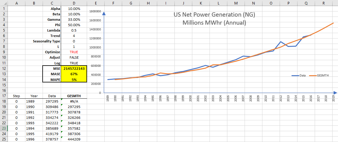

Finale:

That’s all for now, thank you for watching!