General Exponential Smoothing (GESMTH) with trend, seasonality and Chatfield adjustment.

Scene 1:

Hello and welcome to the exponential smoothing tutorial series. In this part, we’ll introduce our latest addition to the exponential smoothing functions family – The General Exponential Smoothing Function (GESMTH).

The GESMTH not only supports prior smoothing models covered by the Simple, double, and triple exponential smoothing function, but it implements additional types for trend and seasonal components. Furthermore, the GESMTH supports data prior-transformation and Chatfield correction/adjustment for 1st order autocorrelation in the forecast errors. In short, GESMTH is the ultimate tool in our arsenal to exponentially smooth your data, and project forecast.

In this video, we will cover the smoothing models of seasonal and trending data set using the different trend and seasonality types and built-in automatic optimization for the smoothing parameters.

In this video, we will use the monthly net power generation in the US using natural gas (as a fuel) between January 1989 – March 2017. The data was sourced from US Energy Information Agency (aka EIA), and units are expressed in millions of MWhr (Mega Watt Hours).

Scene 2:

Examine the plot of the data over time along with a 24-months moving average, and let’s draw a few observations:
- The time series is definitely exhibiting annual seasonality.
- Although the ups and downs in the signal are changing over time, the time series doesn’t suggest a relationship with levels. In other words, as the level increases, the peaks and troughs are not changing accordingly.
- The level of the net power gen (aka 24-months moving average) is growing approximately in a linear fashion.

Now, we have an idea of what we dealing with, let’s begin! For illustration, we list the input arguments of GESMTH in cells D1-D11. Select cell D18.

Scene 3:

Type in the function name – GESMTH in the cell or in the equation toolbar. Note that the auto-complete feature in Microsoft Excel will help find the correct function.

Scene 4:

Once you find the GESMTH function, click on the “fx” button located on the left of the equation toolbar. This will invoke the “function arguments dialog” for GESMTH.

Scene 5:

First, let’s specify the input cells range.

Scene 6:

Lock the starting cell reference by pressing F4.

Scene 7:

In the order field, specify 1 (or True) for the time order in the series. This designates that the 1st observation in the input series corresponds to the earliest date and/or time in our time series progresses downward.

Scene 8:

For the level-smoothing parameter (aka. alpha), you can type in a value between 0 and 1, leave blank, or reference an existing cell.

In this example, let’s reference the value in D1.

Scene 9:

And, lock the cell reference by pressing F4

Scene 10:

For the trend-smoothing parameter (beta), you can also type in a value between 0  and 1, leave blank, or reference an existing cell.

In this example, let’s reference the value in D2.

Scene 11:

Lock the cell reference by pressing F4.

Scene 12:

For Gamma or seasonality indices smoothing parameters, you may type a value between 0 and 1, leave blank, or reference the existing cell in your worksheet.

For consistency, let’s reference the value in D3.

Scene 13:

Lock the cell reference by pressing F4.

Scene 14:

Now, for the trend damping coefficient (Phi), you may type a value between -1 and 1, leave blank, or reference a cell in your worksheet.

Let’s reference the value in D4.

Scene 15:

Lock the cell reference by pressing F4.

Scene 16:

For the parameter value of Chatfield’s autocorrelation correction term (aka Lambda), you may type a value between -1 and 1, leave blank, or reference a cell in your worksheet. Let’s reference the value in D5.

Scene 17:

Lock the cell reference by pressing F4.

Scene 18:

For trend-type, you need to choose a value from 0 (no trend) to 4 (damped multiplicative), leave blank (aka no trend), or reference a cell in your worksheet.

Again, let’s reference another cell: D6.

Scene 19:

Lock the cell reference by pressing F4.

Scene 20:

For seasonality type argument, you may leave blank (aka non), enter 1, or reference a cell in the spreadsheet.

For consistency with the rest of the arguments, let’s reference D7.

Scene 21:

Lock the cell reference by pressing F4

Scene 22:

For seasonal length, you may leave blank (no seasonality), type in a value (e.g. 12 for monthly data), or reference a cell.

Let’s reference the value in cell D8.

Scene 23:

Lock the cell reference by pressing F4.

Scene 24:

For enabling/disabling the built-in optimizer, you may type in True/False, leave blank (disabled), or reference the value in a worksheet.

Let’s reference the value in D9.

Scene 25:

Lock the cell reference by pressing F4.

Scene 26:

For enabling/disabling Chatfield’s autocorrelation correction, enter a True/False, leave blank, or reference the value in D10.

Scene 27:

Lock the cell reference by pressing F4.

Scene 28:

For prior-data log transform, reference the value in cell D11.

Scene 29:

Lock the cell reference by pressing F4.

Scene 30:

For the forecast time, we will be forecasting the value at the end of the input data. So, set T to zero, or better yet, reference a cell in column A, so we can change it after the end of the input data.

Scene 31:

Lock the cell for column movement, by hitting F4 until the dollar sign is showing at the left.

Scene 32:

For return type, leave blank or type in zero (0) for "forecast".

Then, click OK.

Scene 33:

The function returns #N/A since we don’t have enough data.

Scene 34:

Copy the formulas to the cells below it, even after the end of the sample data. Don’t worry about the empty cells picked up after the end of the input data, the function will ignore them.

Scene 35:

Before we can compare other smoothing models, let’s quantify the forecasting accuracy of the new series. For this illustration, we will use three forecast performance measures: for an absolute measure, we will use mean-squared-error (MSE), for percentage error, we choose symmetric mean absolute percentage error (MAPE), and for a relative scaled error (relative to seasonal-naïve model (i.e. period=12 month)), we will use the mean absolute scaled error (MASE). Those functions are part of NumXL and are available as worksheet functions.

Scene 36:

First, let’s examine a no-trend model and no-seasonality (aka Brown’s simple exponential smoothing). Set the trend type to 0 (i.e. no trend) in D6, and seasonality-type to 0 in D7. Leave the value in D8 intact, as GESMTH will simply ignore it. The worksheet auto-calculates all values, and the plot reflects the new series. It does not look very good.

Looking further to the forecast accuracy measure:
- MASE states it performs worse than plain naïve forecast (29% worse).
- MAPE shows that the average percentage error is around 14%.

Scene 37:

Before we can examine seasonal models, let’s decompose the smoothed signal (and forecast) into Level-Trend and Seasonal Indices, to better understand the fit of each model. Copy the formula in D18 to E18, select E18, and press the “fx” button (left of equation toolbar). Change the input cells range, to cover all inputs from C18-C356. Press F4 to lock the whole cells range. Change the forecast time/horizon input to a value equal to the number of steps for our forecast beyond the end of the input cells range. For our illustration, we are forecasting 41 months post march 2017. Press F4 to lock the cell. Finally, change the return type from 0 (or blank) to 6 for the level component. Click OK.

The function returns #N/A. This is OK as this is the 1 st value in the array. Now, starting from cell E18, select all cells up to E397. Press F2, to edit the formula. Press CTRL + SHIFT + ENTER (Control + Shift + ENTER/RETURN). This will populate the level values. Repeat the same steps for Trend and Seasonal Indices in column F + G. Notice both series returns #N/A, as we don’t have trend or seasonality specified in the model yet. Plot the Level, Trend, and Seasonal Indices in your worksheet.

Scene 38:

OK, let’s add an additive seasonality component. Set the seasonality type to 1 in D7.

Scene 39:

Again, the worksheet recalculates all forecast values, and the graph is updated. It looks better than earlier.

Examining the accuracy measure:
- MASE shows it performs better than the naïve model (31% better)
- MAPE shows the better average absolute error (8% from 14%).

Let’s Examine visually the forecast; The forecast seems to fit the data, okay, and the out-of-sample forecast looks somewhat low.

Scene 40:

Let’s examine both the level and seasonality components for stability. The seasonal component looks stable over the duration of the sample and the forecast horizon. The level component is a bit noisy. This is a good start.

Scene 41:

Now, let’s include an additive trend-type into the model. Set the value in D6 to 1.

Scene 42:

Once Excel recalculates the worksheet, let’s examine the results. The MASE has improved 8%, the MAPE remains the same at 8%.

Scene 43:

Let’s examine both the level and seasonality component for stability The seasonal component looks stable over the duration of the sample and the forecast horizon Trend and Level components look noisy. Nevertheless, this is an improvement.

Scene 44:

How about a damped-additive trend? Change the trend-type in D6 to 2.

Scene 45:

Once excel finishes the recalculation, let’s examine the results: The MASE got worse: actually 3% worse than earlier case.

Scene 46:

Let’s examine both the level and seasonality component for stability The seasonal indices component exhibit variations over the duration of the sample and the forecast horizon. This is not good. Trend converges to zero and stays zero after that. The level is a bit noisy. This is not an improvement.

Scene 47:

Change the trend-type back to additive. Set the value in D6 to 1.

Scene 48:

How about a multiplicative seasonality? Set the seasonality-type value equals 2 in cell D7.

Scene 49:

After the worksheet completes its automatic calculation. Notice that accuracy measure – MASE - got worse

Scene 50:

Also, examine the components, and notice seasonal indices variation throughout the sample. This is not an improvement.

Scene 51:

Set the seasonality type to additive, by setting the value in D7 to 1.

Scene 52:

Now, let’s attempt to use the log-transform for the data. Set the value in D11 to True (or 1).

Scene 53:

After the worksheet calculation is complete, notice that accuracy measures – MASE go better (71%), while the MAPE is back to 8%.

Examine the components of the series, the level looks a bit noisy, but seasonal indices look stable throughout the sample and forecast horizon.

Scene 55:

Now, let’s try a damped-additive trend. Set the value in D6 to 2.

Scene 56:

Hmm... The accuracy measure did not change much, but the out-of-sample forecast is not trending.

Scene 57:

There is one more parameter we have not used so far, Chatfield’s correction. Chatfield correct for 1st order autocorrelation in the model’s forecast values. Let’s try to use it. Set the Log transform back to False (or 0) to disable. Set the trend-type back to additive: enter 1 in cell D6

Scene 58:

Set the Chatfield correction/adjustment term to True (or 1) in cell D10

Scene 59:

Once the worksheet recalculation is complete, notice how the MASE and MAPE have both improved significantly. This is an improvement.

Scene 60:

Let’s examine the components: Level and trend look noisy, and seasonal indices are stable.

Scene 61:

Let’s examine the out-of-sample forecast pattern: The model projects a change in general levels going forward. How reasonable is that? A subject matter intuition is key here!

Scene 62:

Let’s assume we disagree with the model earlier, so let’s choose a different one. Set the trend-type to multiplicative, by setting the value in D6 to 3

Scene 63:

Wait for the worksheet recalculation to complete, then examine the outputs:
- The forecast accuracy remains at the same levels: MAPE 7% and MASE 62%, which is good.
- The level and trend components are relatively smooth and stable.
- The seasonal indices vary throughout the sample, but yet stable
- The out-of-sample forecast projects a growth in the general levels.

Can you combine log transform with Chatfield’s correction? You bet, but we’ll leave this to you to experiment on your own.

Scene 64:

NumXL takes all the numbers crunching heavy-lifting, so you – the subject-matter expert – have the time to exercise your intuitions to filter through the different alternatives, and arrive at the one that makes the best sense to you. Where do we go from here? In this tutorial, we only looked at the general exponential smoothing of one time series with one seasonal pattern. Many time series found in practice exhibit several distinct seasonal variations, for instance, for power demand; it shows daily, weekly, and seasonal patterns. Furthermore, we have not included any exogenous factors; for instance; fuel price level? Available power gen capacity for NG and/or other sources (e.g. Hydro, Wind, Coal, etc.)?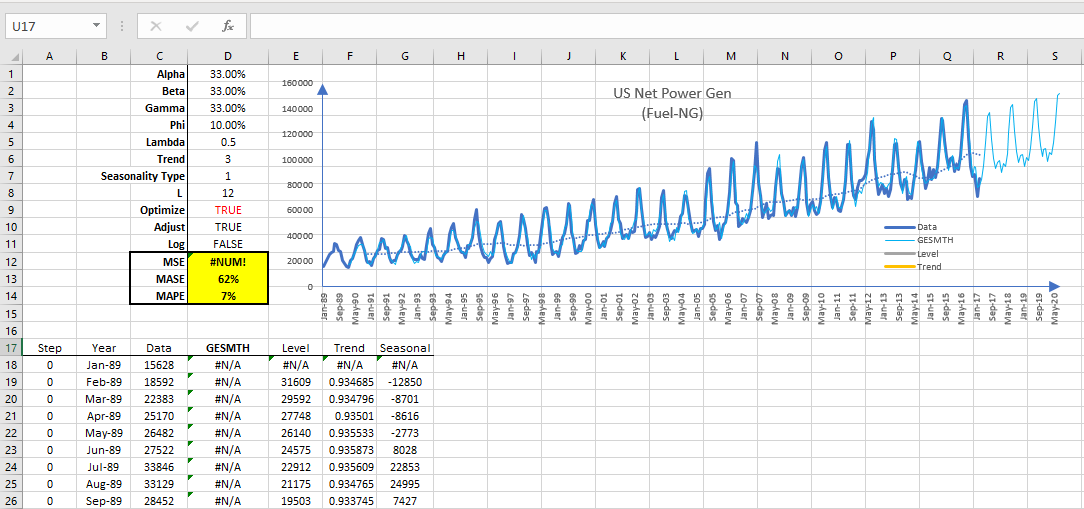

Finale:

That’s all for now. Check with us, later, with updates and enhancements to our smoothing model. Thank you for watching.