Backtesting for X-13ARIMA-SEATS

We hear a lot of questions from our users about forecasting accuracy: How will my model forecast fare with actual future values? Do the forecast values and actuals track closely? What kind of tracking error would it have?

The backtesting technique addresses these questions, with a simple twist: If we were to go back in time, we could calibrate the model using only the data available up to that time and carry out an out-of-sample forecast. Then, we repeat the procedure for different dates.

By the end of the backtesting process, we generate a time series of the forecasted values, which we can then analyze in relation to the actuals time series. Then, we can calculate all sorts of statistics.

This article was inspired by a specific support inquiry from one of our users:

“How can I conduct backtesting on the X-13ARIMA-SEATS forecast of the seasonal adjusted and final (i.e., non-seasonal adjusted) values?”

To carry out the backtesting, we’d need to run several X13AS scenarios that only differ by the input data set.

For this tutorial, we’ll use the non-farming payroll employment monthly data from the U.S. Department of Labor (DOL) between Jan 1970, to June 2022.

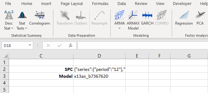
1. Using the X13 Wizard, construct the X13 model using the full data set. The wizard will write the model specification (JSON text) into your worksheet where you specify it.
   
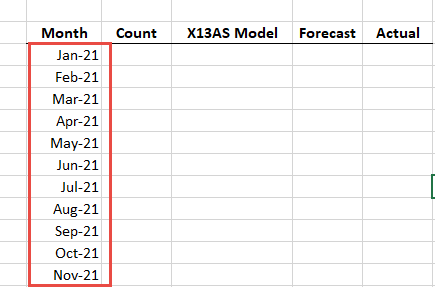
2. Next, in an empty column, list all periods you wish to do a forecast for.
   
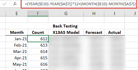
3. Calculate the number of data points from the start of the dataset to each period specified in step (2).
   
4. Copy the X13AS(.) formula in (1) in a separate column, adjacent to the column from step (3).
   
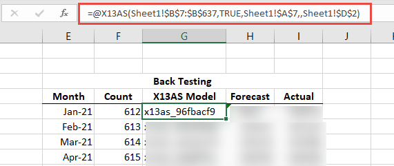
5. Replace the cells-range of the input data with a call to NxSubset(.). The NxSubset function will take the full dataset as its 1st argument, but the finish offset is calculated in the column from step (3).
   

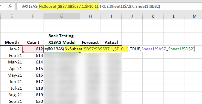
   Note:

   Please refer to the NxSubset(.) Reference Manual page to learn more.

6. Now, the X13AS(.) function constructs a new scenario using only data up to this point.
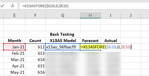
7. Using the X13ASCOMP(.) and X13ASFORE(.) functions, query the component or the forecast value for the date on this row.
   
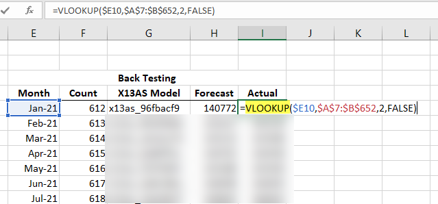
8. Use the Excel built-in function VLOOKUP(.) to query the actual value of each row.
   
9. Copy the formulas from the top row to the rest of the table. This will trigger a series of X13 model calculations, and it may take up to a minute to complete.
   
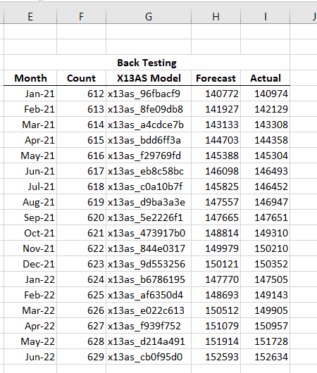
10. Finally, let’s plot the backtesting values alongside the actual values.
    

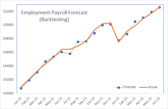
Conclusion

In our example, we calculated the non-seasonal adjusted one-month forecast for the past 24 months, but we can easily expand the study span and/or calculate different outputs.

Once we calculated the backtesting output time series, we should quantitatively describe the forecast tracking error using your favorite forecast performance measure (included with NumXL), such as MAPE, RMSE, MASE, etc.